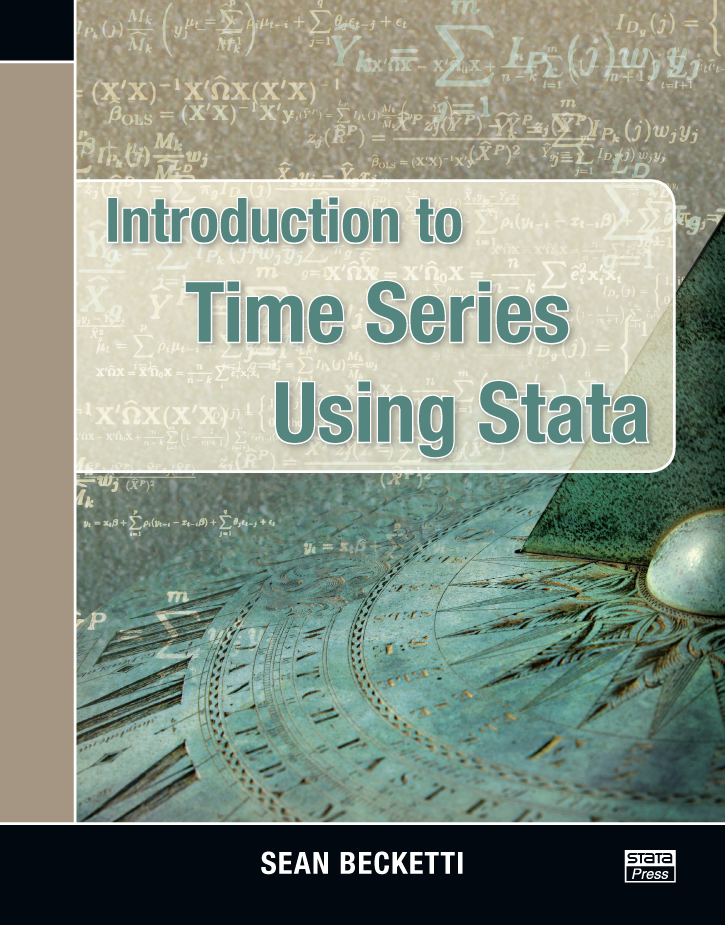
Introduction to Time Series Using Stata, Revised Edition

Introduction to Time Series Using Stata, Revised Edition, by Sean Becketti, is a practical guide to working with time-series data using Stata. In this book, Becketti introduces time-series techniques—from simple to complex—and explains how to implement them using Stata. The many worked examples, concise explanations that focus on intuition, and useful tips based on the author’s experience make the book insightful for students, academic researchers, and practitioners in industry and government.

Becketti is a financial industry veteran with decades of experience in academics, government, and private industry. He was also a developer of Stata in its infancy and has been a regular Stata user since its inception. He wrote many of the first time-series commands in Stata. With his abundant knowledge of Stata and extensive experience with real-world time-series applications, Becketti provides readers with unique insights and motivation throughout the book.

For those new to Stata, the book begins with a mild yet fast-paced introduction to Stata, highlighting all the features you need to know to get started using Stata for time-series analysis. Before diving into analysis of time series, Becketti includes a quick refresher on statistical foundations such as regression and hypothesis testing.

The discussion of time-series analysis begins with techniques for smoothing time series. As the moving-average and Holt–Winters techniques are introduced, Becketti explains the concepts of trends, cyclicality, and seasonality and shows how they can be extracted from a series. The book then illustrates how to use these methods for forecasting. Although these techniques are sometimes neglected in other time-series books, they are easy to implement, can be applied quickly, often produce forecasts just as good as more complicated techniques, and, as Becketti emphasizes, have the distinct advantage of being easily explained to colleagues and policy makers without backgrounds in statistics.

Next, the book focuses on single-equation time-series models. Becketti discusses regression analysis in the presence of autocorrelated disturbances as well as the ARIMA model and Box–Jenkins methodology. An entire chapter is devoted to applying these techniques to develop an ARIMA-based model of U.S. GDP; this will appeal to practitioners, in particular, because it goes step by step through a real-world example: here is my series, now how do I fit an ARIMA model to it? The discussion of single-equation models concludes with a self-contained summary of ARCH/GARCH modeling.

In the final portion of the book, Becketti discusses multiple-equation models. He introduces VAR models and uses a simple model of the U.S. economy to illustrate all key concepts, including model specification, Granger causality, impulse–response analyses, and forecasting. Attention then turns to nonstationary time-series. Becketti masterfully navigates the reader through the often-confusing task of specifying a VEC model, using an example based on construction wages in Washington, DC, and surrounding states.

Introduction to Time Series Using Stata, Revised Edition, by Sean Becketti, is a first-rate, example-based guide to time-series analysis and forecasting using Stata. This is a must-have resource for researchers and students learning to analyze time-series data and for anyone wanting to implement time-series methods in Stata.